Giorgio Giorgiani
Applied Mathematician at ITER
Tel: +33 (0)6 95 39 38 17

Degree-adaptive computations with hybridizable discontinuous Galerkin methods
Discontinuous Galerkin methods (DG) are finite element methods that are locally conservative and stable, and allow to achieve high order accuracy. The interest in DG methods has increased in the last years since they proved to be suited for the construction of robust high-order numerical schemes on arbitrary unstructured and non-conforming grids, for a variety of physical phenomena. The hybridizable discontinuous Galerkin method is a novel DG method with interesting characteristics. While retaining all the advantages of the common DG methods, HDG allows to reduce the coupled degrees of freedom of the problem to those of an approximation of the solution defined only on the faces of the mesh. Moreover, the convergence properties of the HDG solution allow to perform an element-by-element postprocess resulting in a superconvergent solution. I proposed an adaptive technique based on the local variation of the polynomial of interpolation in each element. The superconvergent postprocess is used to define a reliable and computationally cheap error estimator, that is used to drive the automatic adaptive process. The polynomial degree in each element is automatically adjusted aiming at obtaining a uniform error distribution below a user defined tolerance. Since no topological modification of the discretization is involved, fast adaptations of the mesh are obtained.
Adaptive computation are particularly suited for moving geometries and reference frames. In fact, in this situations no a priori adaptation of the computational mesh is possible, and the complex flow structures cover, in different time instants, all the mesh. In this example, the adaptive technique has been used to compute a wind turbine in 2D.
The upper figure shows the vorticity while the bottom figures shows the map of interpolation degrees in the same instant of time.
A video of the vorticity field is available.


In the following example I computed the flow around a NACA0012 airfoil in laminar regime at Re=5000. The upper figures show the velocity magnitude with zoom in the leading edge and the trailing edge. The recirculation bubbles are also highligthed. The bottom figures show the map of polynomial interpolation degrees.


A 3D example is also proposed in my thesis, that is, the solution of a cavity problem. In the following figures, the isosurfaces of velocity and the map of polynomial degree is shown for Re=1000.


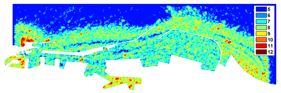
I applied the degree-adaptive technique also to wave propagation problems. Using the Mild Slope equation, I computed the sea wave distribution in the Barcelona harbor. The solution and the degree-distribution in the computational domain are shown below. For the exterior boundary, a Perfectly Matched Layer is used to avoid spurious wave reflections inside the domain.

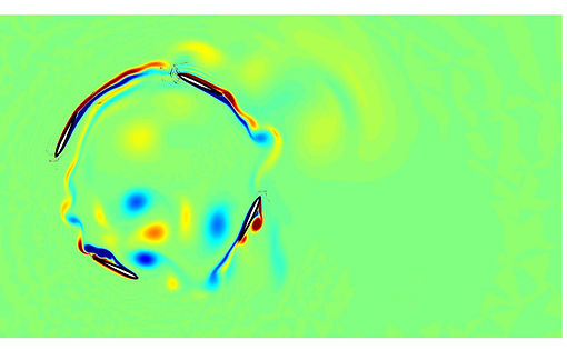
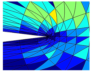
In the next example it is studied the periodic vortex shedding flow past a unitary radius cylinder at Re=100. The figures show the vorticity magnitude (left) and the degree map (right), just before and after the start of the vortex shedding. In the video is shown the evolution of the simulation.
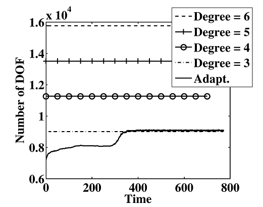
The next figure depicts the variation in time of the number of DOF of the adaptive computation, compared with the constant DOF of the uniform degree computations. . For the adaptive simulation, three different phases can be identified. First the number of DOF increases smoothly and reaches a constant value. In this part of the simulation, the cylinder is not shedding and the adaptive technique is placing high-order elements around the cylinder and in the recirculation zone behind it. The rapid increase in the number of DOF around time t = 300 corresponds to the start of the shedding pattern.
Finally, the table shows the error in the mean drag force on the cylinder, averaged in one period of the periodic shedding regime, for the adaptive computation and for uniform degree computations with k = 3, 4, 5. Since the adaptive computation never requires elemental degrees larger than 6 in any element, the mean drag force for the uniform degree computation with k = 6 is considered as reference value. The adaptive simulation provides the best accuracy, with the minimum number of DOF.